Directions
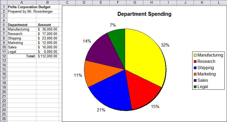
Use the following guidelines to create a pie chart of departmental spending at Pella Corporation.
- Create a new spreadsheet. In cell A1, type “Pella Corporation Budget” in bold text.
- In cell A2, type “Prepared by” with your name. Save with the name Department.
- In cells A5-B5, type the column headings “Department” and “Amount” in bold text. Add a bottom border.
- Add the six departments shown in the example and the amount budgeted for each. Add a bottom border below row 11. Resize columns as necessary.
- In row 12, add a total using a function as shown in the example.
- Highlight cells A5:B11 and click the Chart Wizard button.
- Step 1: Select “Pie” chart type and use the Normal (not 3D)type. Click Next.
- Click on Step 4: “Chart Elements” and set the chart title to “Department Spending” before clicking Finish.
- Double click on the chart, the right-click in near the center of your pie chart and choose “Insert Data Labels,” then right-click again and choose “Format Data Labels.” Then select “Show value as percentage” and deselect “Show value as number”.
- Change the page orientation to landscape. Page preview and return to the normal view.
- Using the handles, resize the chart so that it fills the remainder of the page and everything fits on one page. Page preview again to verify that it fits and fills the page.
- Save the modified file.
- Raise your hand and ask your teacher to grade your spreadsheet on screen.
Example

